Tesseract Hackathon 2026 · Track: multi-physics & coupled systems · Apache-2.0
Coldplate
One jax.grad across three languages, four derivative stacks
and a two-way physics loop — and the loop is the part everyone else drops.
The result
Temperature drives the flow through buoyancy and the flow drives temperature through advection, so the steady state is a fixed point rather than a chain. Cutting that loop — the shortcut written whenever one solver hands out no derivatives — is not a small approximation. It is most of the gradient, and the forward solution gives no warning at all.
| what was measured | result |
|---|---|
| the loop-cut gradient, against a true coupled finite difference | relative error 85.6%, cosine 0.5335, 33% of design variables with the wrong sign |
| the same shortcut with the velocity field frozen | relative error 83.1%, cosine 0.5604, 27% wrong sign |
| acting on each gradient, then scoring both with the true coupled solver | the coupling-complete choice cools by -0.08789 against -0.05565 — 58% more realised cooling at equal raw-variable count and amplitude |
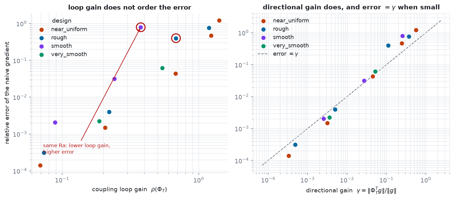
| screening the shortcut for one VJP | log-correlation 0.995 between γ and the error over 14 converged configurations, against 0.825 for the spectral radius |
measured in results/gradient_validation.json · results/intervention_test.json · results/predictor_statistics.json
Who this is for. Anyone standing in front of a coupled pipeline deciding whether to build the coupled adjoint or just differentiate the components separately — conjugate heat transfer, fluid–structure interaction, reservoir–geomechanics, any two solvers that feed each other. That call is usually made on intuition, because the forward solution looks healthy either way. This project measures what the shortcut actually costs on one such problem, shows that the obvious diagnostic is not sufficient, and ships the one-VJP screen that works better as a module that knows nothing about cold plates.
What is composed
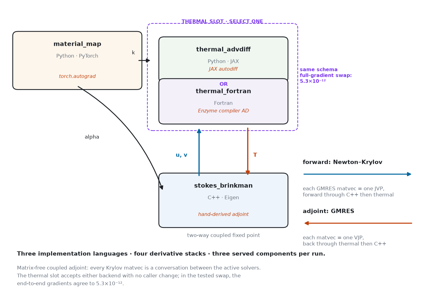
Three implementation languages and four derivative stacks. Three containers are served in any one run: the material map, the fluid solver, and exactly one of the two interchangeable thermal backends.
| Tesseract | language | how derivatives are obtained | role |
|---|---|---|---|
stokes_brinkman | C++ / Eigen | hand-derived discrete adjoint, no AD tool | served |
thermal_advdiff | Python / JAX | JAX autodiff of the residual | served (thermal slot) |
thermal_fortran | Fortran | Enzyme, compiler AD over LLVM IR | served (thermal slot) |
material_map | Python / PyTorch | torch.autograd | served |
The forward solve is Newton–Krylov on
F(T) = Φ(T) − T; the gradient is a GMRES solve against
(I − ΦT)T. Every matvec in both crosses the
container boundary — a JVP forward through the C++ block then the thermal block, a
VJP backward through the thermal block then the C++ block. That is the sense in which
the composition is load-bearing rather than convenient: there is no ordering of these
components in which one sweep of the chain rule suffices.
Chain, unrolled loop, solved loop. “Two-way coupled” covers three different things. A chain needs one sweep of the chain rule. An unrolled loop contracts, so you iterate a fixed number of times and differentiate through the iterations — exact for the iterate it computes, no adjoint solve needed, and the right choice when the loop contracts and the coupled state is small. This is the third kind. At the gradient-study state ρ(ΦT) ≈ 1.19 > 1, so the Picard iteration you would unroll does not converge at all — ours did not, and Anderson acceleration did not rescue it — and the coupled state is a temperature field carrying N² unknowns rather than a handful of scalars. The steady state has to be solved for, by Newton, and its sensitivity by a second transposed solve whose operator exists only as an action across the container boundary.
The two thermal backends share a schema and nothing else, and they are interchangeable rather than merely composable. Swapping JAX autodiff for the independently written Fortran differentiated by Enzyme, at a converged coupled state on a 16×16 grid:
| level | JAX vs Fortran/Enzyme |
|---|---|
component T | 7.1 × 10⁻¹⁶ |
| component JVP | 1.4 × 10⁻¹⁵ |
| component VJP | 4.3 × 10⁻¹⁵ |
converged coupled state T* | 4.8 × 10⁻¹² |
end-to-end dJ/dρ | 5.3 × 10⁻¹², cosine 1.000000000000 |
The gradient that comes out of the whole composition — through the C++ fluid
solver and the PyTorch material map — does not care whether the thermal block was
differentiated by a Python tracer or by a compiler pass over Fortran. Reproduce it with
python orchestrator/compare_thermal_backends.py 16, which writes
the file these numbers are read from.
measured in results/thermal_backend_parity.json
The gradient changes a realised engineering decision
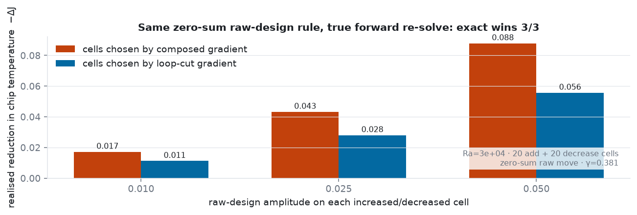
Gradient accuracy only matters if acting on it changes the physical outcome. At a strongly coupled state each gradient was given the same rule — raise the 5% of design variables it calls most beneficial, lower the 5% it calls least beneficial by the same amplitude, zero-sum in the raw variables — and then both predictions were thrown away and the true coupled forward problem re-solved. Filtering and projection are nonlinear, so this equalises the raw move, not the realised density move.
| raw amplitude per selected cell | ΔJ, cells chosen by the exact gradient | ΔJ, cells chosen by the loop-cut gradient | extra realised cooling |
|---|---|---|---|
| 0.010 | -0.01715 | -0.01121 | 53% |
| 0.025 | -0.04322 | -0.02800 | 54% |
| 0.050 | -0.08789 | -0.05565 | 58% |
measured in results/intervention_test.json
Repeated over a frozen 48-attempt matrix
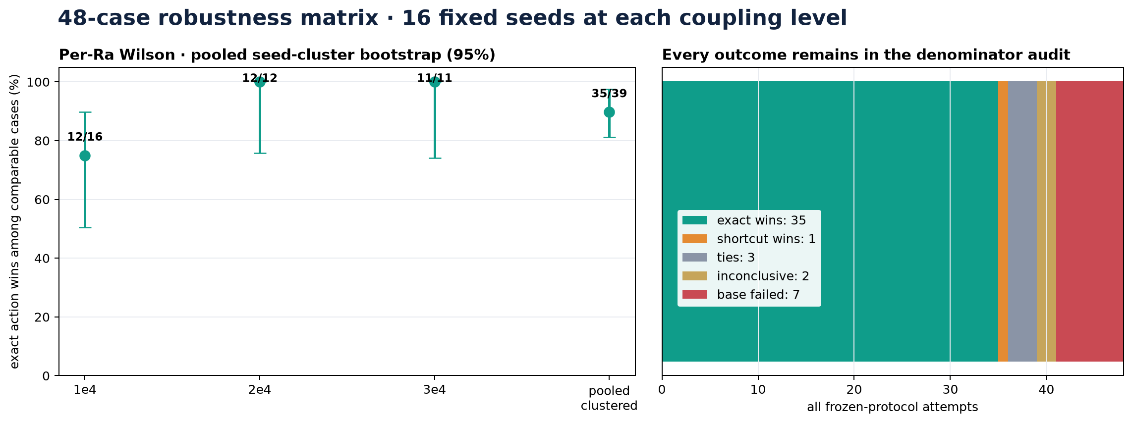
The retrospectively frozen extension completed every planned
(Ra, seed) cell and kept base-solver failures, incomplete action pairs, ties
and the one shortcut win. It is a robustness extension rather than an untouched
independent confirmation set: 13 of the 48 cells had stored evidence before the
design was frozen, and that split is reported rather than buried.
| Ra | exact wins | shortcut wins | ties | noncomparable |
|---|---|---|---|---|
| 10,000 | 12 | 1 | 3 | 0 |
| 20,000 | 12 | 0 | 0 | 4 |
| 30,000 | 11 | 0 | 0 | 5 |
| pooled | 35 | 1 | 3 | 9 |
35 of 39 comparable cases (89.7%) favour the exact-gradient action; the attempt-level Wilson interval is 76.4%–95.9%. Because each seed appears at all three Rayleigh numbers, a secondary bootstrap resamples the 16 complete seed clusters rather than pretending the attempts are independent; that post-freeze descriptive interval is 81.1%–97.4%.
measured in results/intervention_robustness_matrix_48.json
One VJP says whether the shortcut is safe
The adjoint solves (I − ΦT)Tλ = g.
Cutting the loop uses λ0 = g, whose residual in that
equation is exactly ΦTTg. Its normalised norm
— the directional gain
γ = ‖ΦTTg‖ / ‖g‖
— costs one VJP, far less than the gradient it screens, and unlike the spectral
radius it knows which direction the objective actually cares about.
| predictor | correlation with log10(loop-cut error) |
|---|---|
| ρ(ΦT), the loop gain | +0.825 |
| log10(γ), the directional gain | +0.995 |
Over 14 converged configurations drawn from 4 design families and 5 Rayleigh levels. Leave-one-family-out correlations are 0.994–0.997; a seeded 10,000-sample bootstrap gives a 95% interval of 0.989–0.999.
measured in results/predictor_statistics.json · results/predict_error.json
The confound removed: hold the physics fixed, change only the objective
At one design and one Rayleigh number there is a single coupled state, hence a single
ρ(ΦT) = 0.5481 on every row below. Changing what is being measured
changes g = dJ/dT, and therefore γ — but ρ cannot move. The
error still varies by a factor of 136×, so a constant cannot explain it.
| objective | γ | loop-cut relative error |
|---|---|---|
| outlet mean | 0.0027 | 0.0117 |
| top half mean | 0.0076 | 0.0026 |
| chip peak | 0.0261 | 0.0385 |
| chip mean | 0.0300 | 0.0399 |
| domain mean | 0.0967 | 0.0211 |
| left column mean | 0.3879 | 0.3535 |
γ moves with the error and gets the dangerous row right, but it is a screening
signal with a theoretical basis, not a formula: across objectives it correlates 0.80
against 0.995 across designs, because converting an adjoint-equation residual into a
design-gradient error also involves
(I − ΦTT)−1.
measured in results/objective_sweep.json
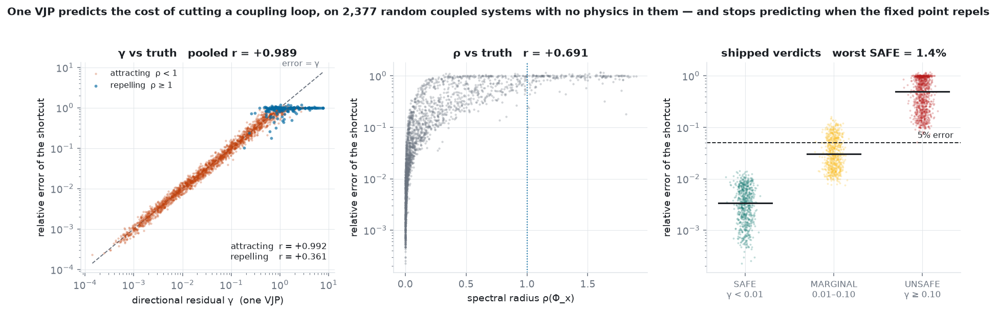
Does it generalise off this problem? 2,377 random systems
The physics is removed entirely: random coupled fixed points
x* = Φ(x*, θ) where every quantity is closed form — no solver
tolerance, no finite differences — across four structural families and both linear
and nonlinear loops, with γ computed by calling the shipped
coupling_check.py rather than a reimplementation.
| subset | n | corr(log γ, log error) | corr(ρ, log error) |
|---|---|---|---|
| all | 2,377 | +0.9893 | +0.6907 |
| lowrank | 600 | +0.9900 | +0.7159 |
| nonnormal | 579 | +0.9817 | +0.6502 |
| normal | 600 | +0.9957 | +0.7979 |
| sparse | 598 | +0.9945 | +0.7222 |
| linear loops | 1,906 | +0.9884 | +0.6923 |
| nonlinear loops | 471 | +0.9935 | +0.7095 |
The shipped thresholds hold, which matters more than the correlation, because a false SAFE is the verdict that hurts someone — it tells them to skip the adjoint. 656 cases below γ = 0.01 have a worst error of 1.4%, and 100% sit under 5%: no false SAFE. 965 cases above γ = 0.10 are 100% genuinely above 5% error: no false alarm.
And the boundary, which we would rather not have found. γ
correlates +0.9925 on the
2,199 attracting fixed points (ρ < 1) but only
+0.36 on the 178 repelling
ones, because the residual it measures is amplified by
(I − ΦTT)−1 and no
contraction bound applies there. The shipped policy for a repelling fixed point is
therefore to refuse to screen and compute the adjoint — which is exactly what this
project does at its own headline state, where ρ ≈ 1.19.
measured in results/gamma_generalization.json
Move the gate yourself
Every dot is one random coupled system: its directional gain across, the true error of the loop-cut gradient up, both on log axes. Orange dots are the ones where cutting the loop costs more than 5%. A gate is a vertical line, and everything to its left is a system the screen would wave through without an adjoint — so an orange dot inside the shaded band is somebody being told to skip a computation they needed.
Gating at γ < 0.003 screens 294 of the 2,377 systems as safe to differentiate component-wise. Worst true error among them: 0.4%. Above the 5% line: no false SAFE.
Gating at γ < 0.01 screens 656 of the 2,377 systems as safe to differentiate component-wise. Worst true error among them: 1.4%. Above the 5% line: no false SAFE.
Gating at γ < 0.03 screens 1,025 of the 2,377 systems as safe to differentiate component-wise. Worst true error among them: 4.2%. Above the 5% line: no false SAFE.
Gating at γ < 0.1 screens 1,412 of the 2,377 systems as safe to differentiate component-wise. Worst true error among them: 16.2%. Above the 5% line: 229 false SAFE.
Gating at γ < 0.3 screens 1,753 of the 2,377 systems as safe to differentiate component-wise. Worst true error among them: 71.4%. Above the 5% line: 570 false SAFE.
counts recomputed at build time from
results/gamma_generalization_points.json, written by the same run that
produced the summary above. ★ marks the gate coupling_check.py
actually ships.
Validation
The coupled physics reproduces the classical onset of convection
A fluid layer heated from below stays motionless until buoyancy overcomes viscous and
thermal diffusion, at a precisely known Rac = 1707.762 for rigid
walls. Onset is also exactly where this project's own machinery puts it: at the
conduction state the coupling loop is the linear stability operator, so
convection begins precisely when the loop gain reaches one. No-slip side walls stabilise
a confined box, so the measured value must sit above the classical one and fall towards
it as the box widens.
| aspect ratio | Rac measured | excess over 1707.762 |
|---|---|---|
| 1 | 2519.07 | +47.507% |
| 2 | 1970.84 | +15.405% |
| 4 | 1779.02 | +4.172% |
| 8 | 1707.97 | +0.012% |
At aspect ratio 8 that is agreement to four significant figures. One number checks the C++ Stokes solver, the thermal solver, the buoyancy coupling between them and the loop-gain machinery, all at once.
measured in results/critical_rayleigh.json
The discretisation converges at second order
Verification rather than validation: does the code solve its own equations at the rate the scheme implies? Smooth analytic properties, the grid-dependent density filter bypassed, Richardson extrapolation on two independent grid trios — observed order 1.87 and 1.83, monotone in J.
| N | J | converged |
|---|---|---|
| 16 | 3.750196 | yes |
| 24 | 3.762598 | yes |
| 32 | 3.767089 | yes |
| 48 | 3.770452 | yes |
| 64 | 3.771708 | yes |
| 96 | 3.772662 | yes |
measured in results/grid_convergence.json
Nonlinear, finite-Prandtl cavity
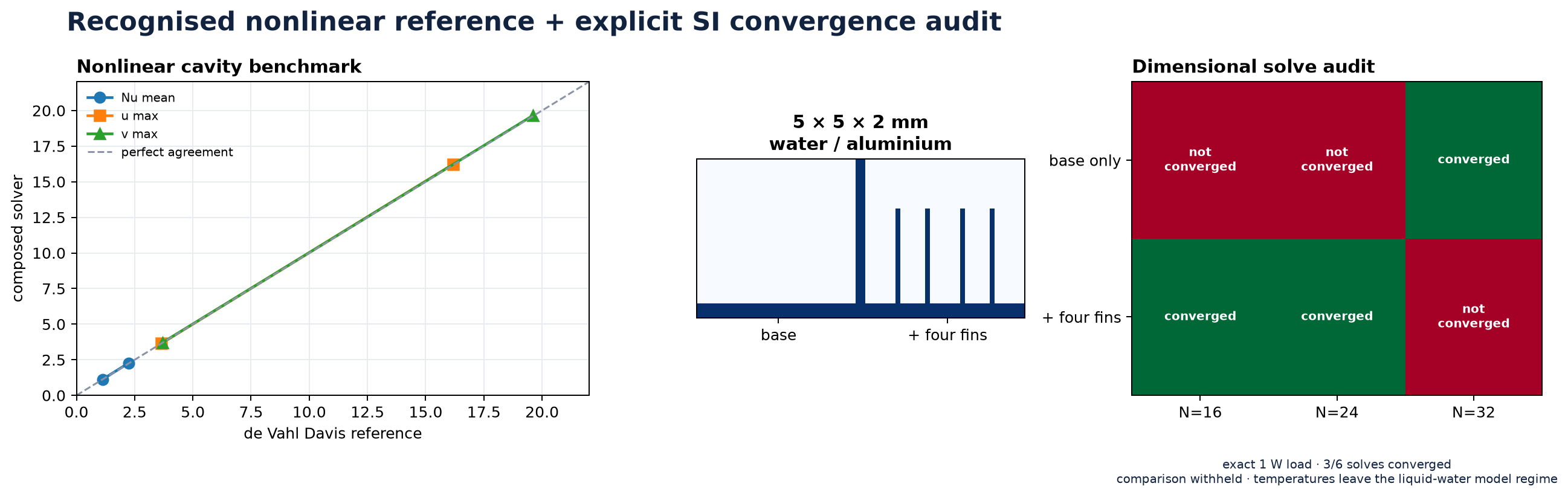
The de Vahl Davis benchmark activates the Navier–Stokes inertia term, so it validates the nonlinear path rather than asking the Stokes approximation to reproduce finite-Prandtl flow. Both cases converge, and all 6 Nusselt and centreline-velocity observables land within 1.2% of the published references.
measured in results/de_vahl_davis.json
Where an unrolled loop is fine, and where it is not
“Two-way coupled” covers three different things: a chain, an unrolled loop, and a solved loop. Only the third needs any of the machinery here, so that claim is worth testing rather than asserting. Same design draw, same three components, same containers — only the Rayleigh number moves. Both candidates are scored against a central difference of the fully solved coupled problem, the one referee sharing no method with either.
| repelling (Ra = 3×10⁴) | contracting (Ra = 103) | |
|---|---|---|
| loop gain ρ(ΦT) | 1.361 | 0.056 |
| plain Picard | 3.03e+01 → 4.74e-02, stalls | 3.03e+01 → 4.38e-12, converges |
| implicit adjoint | 1.27e-05 | 6.44e-07 |
| best unrolled gradient | 4.84e-02 | 5.61e-07 |
| sweeps unrolled | repelling | contracting |
|---|---|---|
| 1 | 6.17e-01 | 5.40e-04 |
| 2 | 4.84e-02 | 3.71e-05 |
| 4 | 3.89e+00 | 5.61e-07 |
| 8 | 3.11e+01 | 6.44e-07 |
| 16 | 2.87e+00 | 6.44e-07 |
Read the right-hand column first. Where the loop contracts, differentiating the unrolled iteration is as accurate as the implicit adjoint — 5.6e-07 against 6.4e-07. If your loop contracts, unroll it; nothing here is needed.
The left-hand column is why this exists. At ρ = 1.36 the plain iteration stalls at 4.7e-02 instead of converging, the gradient differentiated through it is 5% wrong at best, and more sweeps make it worse rather than better — there is no converged iterate to unroll toward. The implicit adjoint lands at 1.27e-05, about 3,795× closer.
measured in results/unroll_study.json
What Tesseract's own gradient checker found
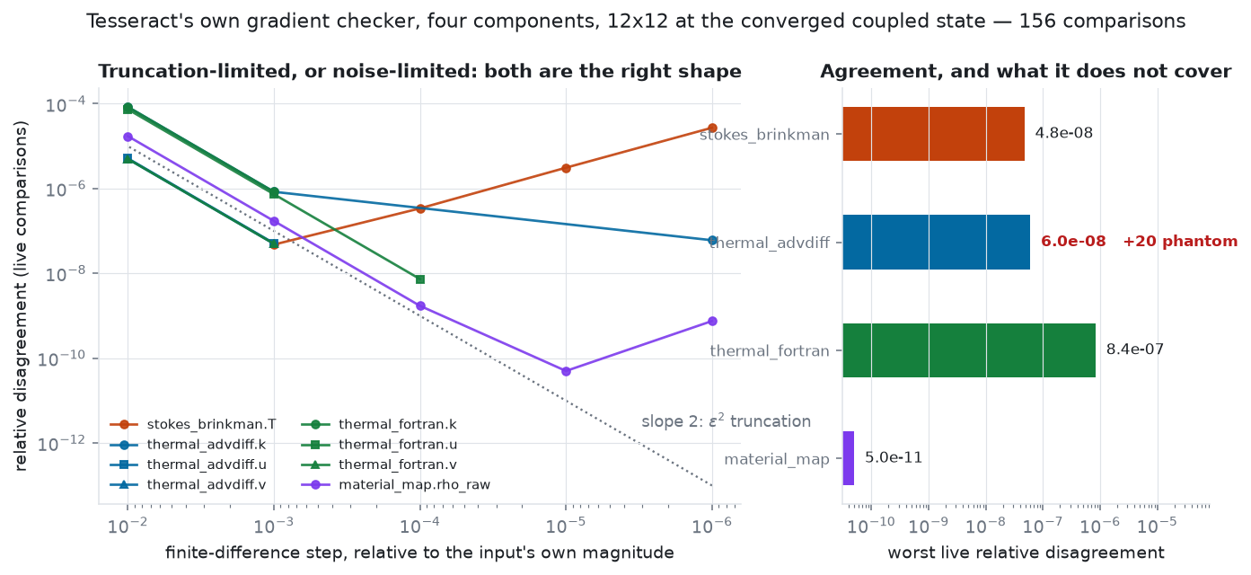
Every other check on this page is one we wrote. Tesseract ships its own: it samples
random input/output index pairs and compares each declared derivative endpoint against a
central difference taken through apply. It knows nothing about cold plates.
Run against all four components at the converged coupled state, it found two things.
| Tesseract | how its derivatives are obtained | inputs checked | relative disagreement | phantom |
|---|---|---|---|---|
stokes_brinkman | C++/Eigen, hand-derived discrete adjoint | T, alpha | 4.8e-08 | 0 |
thermal_advdiff | JAX autodiff | k, u, v | 6.0e-08 | 20 |
thermal_fortran | Fortran, Enzyme compiler AD at the LLVM IR level | k, u, v | 8.4e-07 | 0 |
material_map | PyTorch, torch.autograd | rho_raw | 5.0e-11 | 0 |
The live comparisons agree. Across
156 comparisons the worst disagreement between any endpoint
and a central difference is 8.4e-07
relative — four derivative implementations sharing no machinery, measured by
somebody else's tool. Each figure is the best rung of a
5-step ladder of finite-difference steps, and the number
is not a pass at a threshold picked afterwards: the checker's verdict is
allclose(fd, endpoint, atol=1e-8, rtol=r) and neither side depends on
r, so running it at rtol = 0 hands back both rows and
the disagreement follows by arithmetic.
And it found a defect we had not. 20 of the sampled
comparisons are phantom sensitivities: the finite difference is exactly zero
because the forward map never reads the perturbed input, while the endpoint reports a
real number. They are the wall-face velocities — the assembly apply
uses sums fluxes over interior faces only, while the JAX residual the derivative path
differentiates includes wall terms that vanish in value at a no-slip wall but not in
derivative. The independently written Fortran block has none, which localises it; and
swapping that block in moves the end-to-end gradient by only 5.3 × 10⁻¹²,
which bounds what the defect can cost. It is recorded here rather than quietly fixed.
measured in results/check_gradients.json
What the coupled adjoint costs, and what it replaces
If you were not going to build it, the alternatives are the loop-cut shortcut — whose error is the subject of this whole page — or finite differences over the design vector. At 48×48 that is 2,304 design variables and two coupled solves apiece.
| cost of | wall clock | basis |
|---|---|---|
| one coupled solve from cold, 10 Newton iterations | 10.2 s | measured |
| one finite-difference probe — perturb one variable, warm-started | 1.02 s | measured, median of 5 |
| one composed adjoint gradient, 13 JVP + 15 VJP across the boundary | 3.98 s | measured, median of 3 |
| one central-difference gradient, 4,608 coupled solves | 1.3 h | extrapolated |
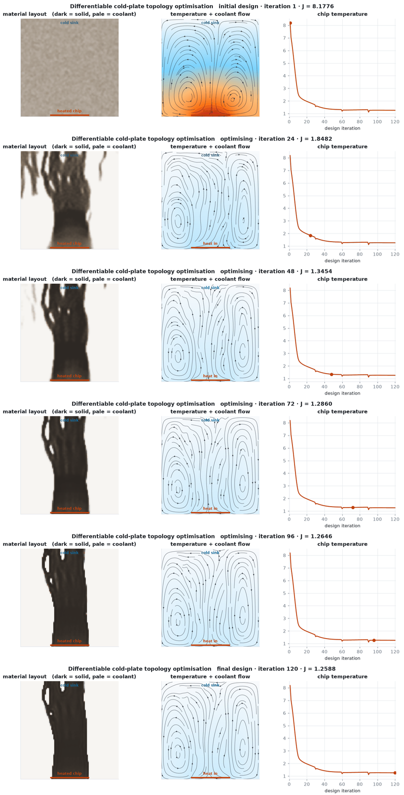
Roughly 1,178×. The per-solve figure is a warm-started probe rather than a cold solve, which is the number most favourable to finite differences. The whole 120-iteration optimisation took 7.8 minutes; on central differences the same schedule extrapolates to 6.5 days. We did not run 4,608 solves to prove a multiplication, and the table says which row was measured and which was not.
measured in results/adjoint_cost.json
What we do not claim
These are the results that did not go our way. They are kept because a study that cannot record a negative is not evidence.
Both gradients drive the long optimisation successfully
Run twice at 96×96 from the same seed and schedule, the coupling-complete and loop-cut gradients reach essentially the same objective — and the naive run ends a hair lower. An optimiser converging is not evidence that a gradient is right. Along that trajectory the shortcut is only 4–20% off with a cosine above 0.98 and almost no sign errors: a perfectly serviceable search direction. Two things differ from the strongly coupled state above — the Rayleigh number, and the fact that filtered, projected designs are smooth while the random design used for the gradient study is not.
Serviceable as a direction, worthless as an attribution
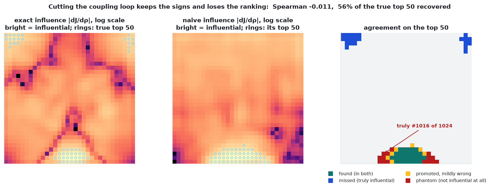
Descent needs only a positive inner product with the truth. Attribution — which parts of the design actually drive the objective, the question behind tolerancing, sensor placement and mesh refinement — reads the gradient entry by entry, so every entry has to be right on its own. Ranking every design cell by influence, the loop-cut ordering of magnitudes correlates -0.011 with the true one: statistically indistinguishable from chance. Its single most influential cell is truly the #4; it recovers 70% of the true top ten and 56% of the true top fifty; and it promotes into its own top fifty a cell that is truly ranked #1,015 of 1,024 — among the least influential in the entire domain. Sign agreement on the cells that genuinely matter is 100%. Signs survive; magnitudes do not, and nothing in the forward solution would warn the engineer who tightened a tolerance on that cell.
measured in results/sensitivity_ranking.json
The frozen eight-step showdown did not complete
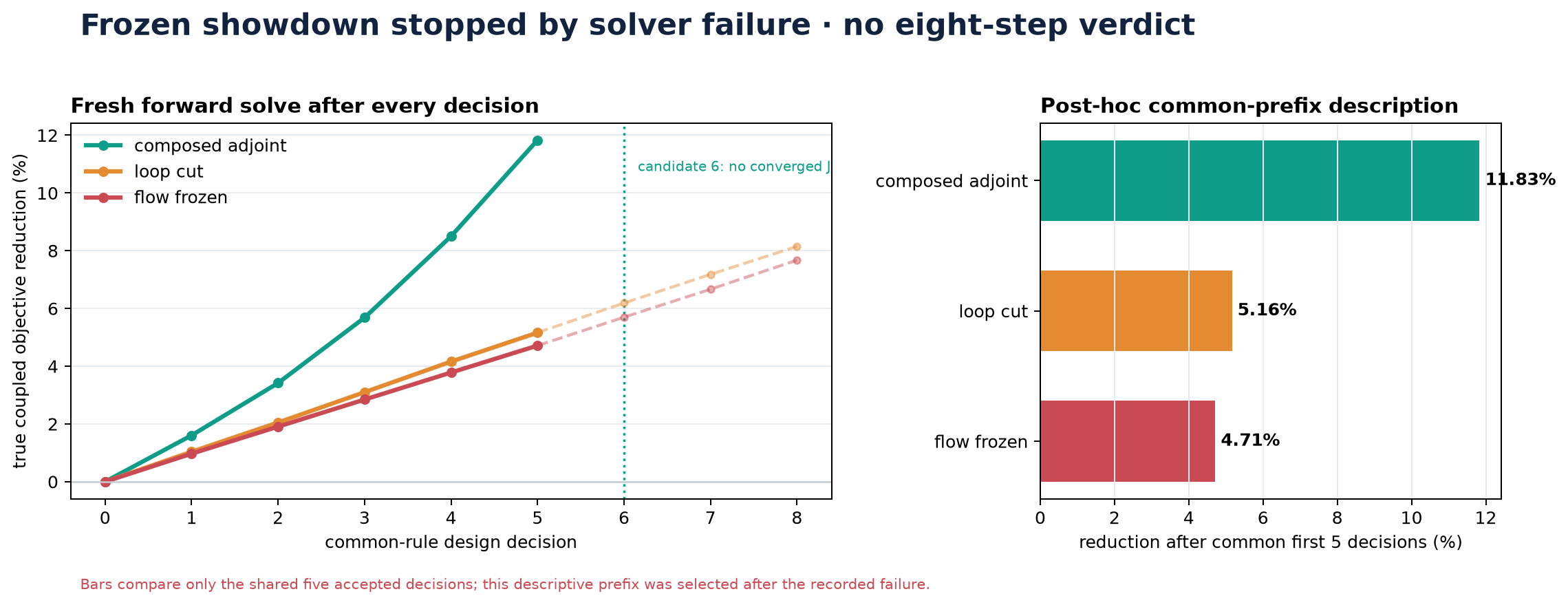
Three branches were given the same initial design, proposal rule, projected-volume target, eight update opportunities and candidate-solve budget. The composed branch accepted five decisions and then its sixth candidate failed to converge inside the frozen budget. Because the horizons differ, the eight-step endpoint is not evaluable and there is no verdict. The shared five-step prefix — 11.83% composed, 5.16% loop-cut, 4.71% frozen-flow — was examined after the failure; it is descriptive context, not the frozen endpoint, and it is not called a win.
measured in results/strong_coupling_showdown_interpretation.json
The dimensional SI example is a failed audit
Only 3 of 6 planned layout and mesh solves converged, and even the converged baseline temperature sits outside the constant-property liquid-water regime the model assumes. Its apparent resistance reduction is withheld rather than reported. The exact bookkeeping, the solver outcomes and the failure all remain stored, and the script exits non-zero on this condition rather than printing a number.
measured in results/dimensional_coldplate.json
And the scope
This is a steady two-dimensional research prototype at modest resolution, with no experimental validation, no pressure-drop or manufacturing analysis and no three-dimensional effects. Differentiable topology optimisation of thermo-fluidic devices is not new, and neither is natural-convection heat-sink design; what is new here is composition across genuinely heterogeneous components, the demonstration that spectral radius alone is insufficient for this decision, and γ as an operational one-VJP check.
Reproduce it
Supported review path: Linux amd64, or Windows through WSL2, with a
running Docker daemon and Python 3.12+.
pip install -r requirements-orchestrator.txt
bash scripts/judge_demo.sh        # 1-3 minutes warm: serves both thermal backends
                                  # and swaps them on an 8x8 smoke grid
Then any of:
cd orchestrator
python validate_pipeline.py 16                 # composed gradient vs finite differences
python compare_thermal_backends.py 16          # JAX and Fortran/Enzyme are interchangeable
python sweep_coupling.py                       # where component-wise differentiation breaks
python predict_error.py --N 20                 # what predicts the damage, for one VJP
python gamma_generalization.py --trials 2400   # no containers, no solver, closed-form truth
python intervention_test.py --N 20 --Ra 3e4    # act on each gradient, re-solve the truth
The full command set, including the long optimisations and the frozen protocols, is in
the repository README. The extended evidence is
byte-bound to the workflow runs that produced it in
orchestrator/results/EVIDENCE_PROVENANCE.json, and rechecked with
python scripts/validate_evidence_provenance.py --verify-github.